KMT coupling - animation

mathematical details on the construction of KMT coupling with a JS animation

How do you visualize the diffusion approximation of some random walk? A naive, yet common, answer is to plot the rescaled random walk and hope that the path resembles a Brownian path. This is not satisfactory and this is where KMT coupling comes in.

KMT coupling is one of the central tools behind strong diffusion approximation. It provides a pathwise comparison between partial sums of independent random variables and Brownian motion, with a logarithmic maximal error.

1. What is a diffusion approximation?

Let $(\xi_i)_{i\geq 1}$ be i.i.d., centered, with variance $1$, and define

\[S_k=\sum_{i=1}^k \xi_i.\]

The Central Limit Theorem says that $S_n/\sqrt{n}$ converges in law to the standard Gaussian distribution $\mathcal{N}(0,1)$. Yet it does not say anything about the trajectories of the random walk $(S_k)_{1\leq k\leq n}$. This is where Donsker’s theorem takes over. Let

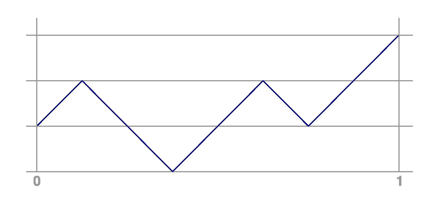
\[X_n(t)=\frac{1}{\sqrt n}\Big(S_{\lfloor nt\rfloor}+(nt-\lfloor nt\rfloor)\xi_{\lfloor nt\rfloor+1}\Big),\qquad t\in[0,1],\]

denote the rescaled interpolation of the random walk. Here is a trajectory of $X_n$ for $n=8$ when $\mathbb{P}(\xi_i=1)=\mathbb{P}(\xi_i=-1)=1/2$.

Donsker’s Theorem. The rescaled process $X_n$ converges in law to a standard Brownian motion $B$ in the space of continuous functions on $[0,1]$.

This is the simplest diffusion approximation result: a random walk can be approximated by Brownian motion.

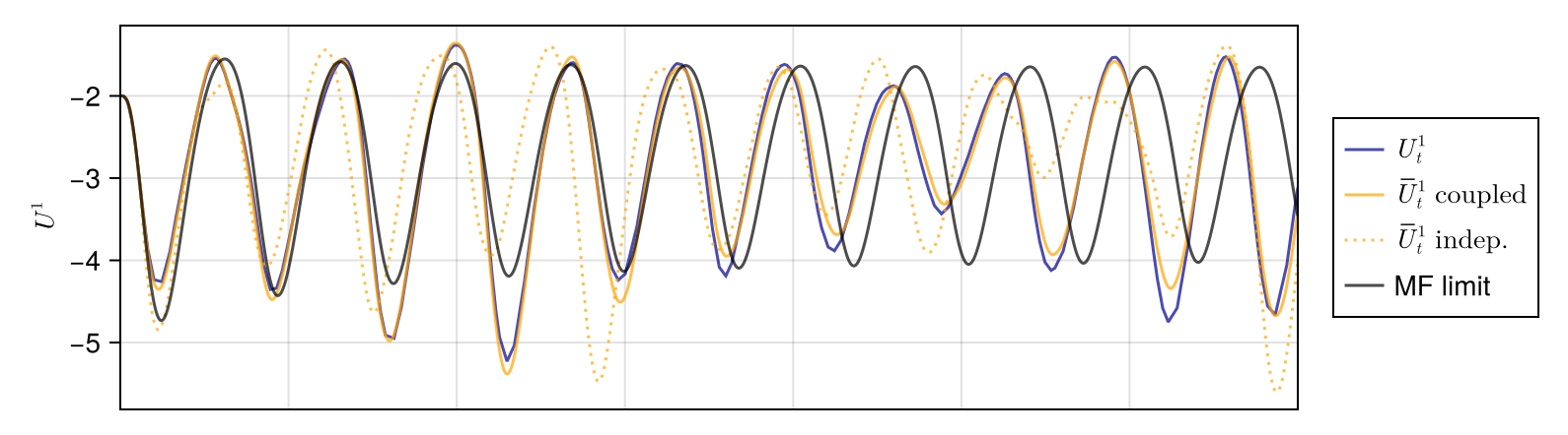
More complex diffusion approximation concerns more general processes (e.g. Markov chains, interacting particle systems, birth-death processes, etc.) and more general diffusions. Here is a plot taken from my HDR manuscript showing the diffusion approximation of interacting neurons. The true trajectory is the blue one, its mean-field approximation is the black curve, and the orange curves depict two realizations of the diffusion approximation: the dashed one is independent from the blue curve, while the solid one is coupled to the blue curve via KMT coupling. The coupled trajectory stays close to the true one much longer. It gives a nice visualization of the power of the diffusion approximation with respect to the mean-field approximation.

2. Why does KMT coupling matter?

KMT coupling gives a strong diffusion approximation result. It builds $X_n$ and $B$ on one probability space with a sharp error control on the full path. Furthermore, the construction is explicit and can be used to answer the first question of this post: how to visualize a diffusion approximation?

The answer is to plot coupled trajectories of $X_n$ and $B$. That is the purpose of this animation.

Notice that there is also a version which gives a strong approximation of the empirical process by a Brownian bridge, which is the key to many results in statistics.

3. What is the KMT theorem?

The idea is to couple the random walk and the Brownian motion in a way that they are close to each other while keeping the correct laws of both processes. The standard form is the following.

KMT Theorem. Assume $\xi_1$ is centered, has variance $1$, and has a finite exponential moment in a neighborhood of $0$. Then one can construct on one probability space:

1. i.i.d. copies $(\xi_i)$,
2. a standard Brownian motion $(B_t)_{t\geq 0}$,

such that for constants $C,K,\lambda>0$ (depending only on the law of $\xi_1$),

\[\mathbb P\!\left(\max_{1\leq k\leq n}|S_k-B_k|>C\log n+x\right)< K e^{-\lambda x},\qquad x\in \mathbb{R},\ n\geq 1.\]

In particular, Borel-Cantelli lemma gives

\[\max_{1\leq k\leq n}|S_k-B_k|=O(\log n)\quad\text{almost surely.}\]

For the rescaled interpolation $X_n$ and Brownian motion $B^{(n)}(t)=B_{nt}/\sqrt{n}$, it rewrites asRequires also some control of Brownian motion's modulus of continuity.

\[\sup_{0\leq t\leq 1}|X_n(t)-B^{(n)}(t)|=O\!\left(\frac{\log n}{\sqrt n}\right).\]

The basic coupling idea behind the KMT construction is quantile coupling.

4. What is quantile coupling?

For one random variable, quantile coupling is canonical. If $F$ and $G$ are two cdfs and $Z\sim\mathrm{Unif}(0,1)$,

\[Y_1=F^{-1}(Z),\qquad Y_2=G^{-1}(Z)\]

is an optimal monotone coupling in many senses.

A naive idea would be to apply quantile coupling to each random variable $\xi_i$ and the corresponding Brownian increment $B_i-B_{i-1}$. However it would not be sharp enough: the error would be of order $\sqrt{n}$ instead of $\log n$.

5. How to get the logarithmic scaling?

The KMT construction applies quantile coupling at all scales of the problem via a dyadic mechanism. Hence, let us assume now that $n=2^m$ for some integer $m\geq 1$. The dyadic construction ensures that quantile coupling errors accumulate across only $m = \log_2 n$ levels, and not across all time steps. In turn, this explains the logarithmic maximal error.

The paragraph below gives a coarse sketch of the construction. It is recommended to look at the animation in parallel. Look at the animation guide if necessary. Furthermore, a more precise description is given in the next section for $n=8$.

The construction starts from the multi-scale given by the successive powers of $2$. In the first (dyadic) level, the interpolation indices are $0, 1, 2, 4, \dots, 2^{m-1}, 2^m$. Quantile coupling is applied to the increments between these interpolation indices.

Then, at each subsequent level, the remaining gaps are filled by some conditional quantile coupling.

6. Toy example

Interested readers are referred to the seminal paper by Komlos, Major and Tusnady or the review paper by Mozgunov et al.. We follow the same notation. Note that the notation $\tilde U$, $\tilde V$ and $Z$ used below are consistent with the ones appearing in the table on the left column of the animation.

In the animation, the random walk is treated as given, and the coupled Brownian motion is reconstructed from it level by level. The toy example below rather explains how they can be constructed simultaneously.

Let $\Phi$ denote the standard Gaussian cdf and $\Phi_j(x) = \Phi(2^{-j/2} x)$ the cdf of $B_{2^j}$ (completed by $\Phi_{-1} = \Phi$ by convention).

Level 1. There are four pairs of increments:

1. $\tilde U_{-1} = S_1 - S_0$ and $\tilde V_{-1} = B_1 - B_0$,
2. $\tilde U_0 = S_2 - S_1$ and $\tilde V_0 = B_2 - B_1$,
3. $\tilde U_1 = S_4 - S_2$ and $\tilde V_1 = B_4 - B_2$,
4. $\tilde U_2 = S_8 - S_4$ and $\tilde V_2 = B_8 - B_4$.

Each $\tilde U_j$ and $\tilde V_j$ is an increment along $2^j$ time steps. They are coupled via four independent uniform random variables $Z_{-1}, Z_0, Z_1, Z_2$ via $\tilde U_j = F_j^{-1}(Z_j)$ and $\tilde V_j = \Phi_j^{-1}(Z_j)$, where $F_j$ is the cdf of $\tilde U_j$.

After Level 1, the values at times $0, 1, 2, 4, 8$ are determined. Two gaps remain:

1. ${3}$ between indices 2 and 4,
2. ${5, 6, 7}$ between indices 4 and 8.

They are filled in the next level.

Level 2. The first gap is cut in two as the two pairs of increments:

1. left pair: $U_{0,2} = S_3 - S_2$ and $V_{0,2} = B_3 - B_2$,
2. right pair: $U_{0,3} = S_4 - S_3$ and $V_{0,3} = B_4 - B_3$.

Each $U_{j,k}$ and $V_{j,k}$ is an increment along $2^j$ time steps. Note that the “left + right” sums (abbreviated as L+R below) are $U_{0,2} + U_{0,3} = S_4 - S_2 = \tilde U_1$ and $V_{0,2} + V_{0,3} = \tilde V_1$. We also consider the “left - right” differences (abbreviated as L-R below):

\[\tilde U_{1,1} = U_{0,2} - U_{0,3} \quad \text{ and } \quad \tilde V_{1,1} = V_{0,2} - V_{0,3}.\]

At each gap, the total increment is already fixed; we only need to decide how it splits into left and right halves. Hence, the idea is to couple the L-R’s by quantiles conditionally on the L+R’s. Moreover, by properties of the Gaussian distribution, the Brownian L-R’s are independent from the L+R’s. For instance, $\tilde V_{1,1}$ is independent from $\tilde V_1$ so that the conditional cdf of $\tilde V_{1,1}$ given $\tilde V_1$ is $\Phi_{1,1}=\Phi_1$.

Formally, $\tilde U_{1,1}$ and $\tilde V_{1,1}$ are coupled via a new independent uniform random variable $Z_{1,1}$, namely $\tilde U_{1,1} = F_{1,1}^{-1}(Z_{1,1} \mid \tilde U_1)$ and $\tilde V_{1,1} = \Phi_{1}^{-1}(Z_{1,1})$, where $F_{1,1}$ is the conditional cdf of $\tilde U_{1,1}$ given $\tilde U_1$. In turn, the two pairs are computed from the L+R’s and the L-R’s as

\[U_{0,2} = \frac{\tilde U_1 + \tilde U_{1,1}}{2},\quad U_{0,3} = \frac{\tilde U_1 - \tilde U_{1,1}}{2},\quad V_{0,2} = \frac{\tilde V_1 + \tilde V_{1,1}}{2},\quad V_{0,3} = \frac{\tilde V_1 - \tilde V_{1,1}}{2}.\]

The second gap is cut in two as the two pairs

1. left pair: $U_{1,2} = S_6 - S_4$ and $V_{1,2} = B_6 - B_4$,
2. right pair: $U_{1,3} = S_8 - S_6$ and $V_{1,3} = B_8 - B_6$,

which gives the L-R’s:

\[\tilde U_{2,1} = U_{1,2} - U_{1,3} \quad \text{ and } \quad \tilde V_{2,1} = V_{1,2} - V_{1,3}.\]

Once again, they are coupled via a new independent uniform random variable $Z_{2,1}$ and the two pairs are computed from the L+R’s and the L-R’s.

After Level 2, the values at times $0, 1, 2, 3, 4, 6, 8$ are determined. Two gaps remain:

1. ${5}$ between indices 4 and 6,
2. ${7}$ between indices 6 and 8.

They are filled in the next and last level.

Level 3. The construction is similar to Level 2. The first gap is cut in two as the two pairs:

1. left pair: $U_{0,4} = S_5 - S_4$ and $V_{0,4} = B_5 - B_4$,
2. right pair: $U_{0,5} = S_6 - S_5$ and $V_{0,5} = B_6 - B_5$;

which gives the L-R’s:

\[\tilde U_{1,2} = U_{0,4} - U_{0,5} \quad \text{ and } \quad \tilde V_{1,2} = V_{0,4} - V_{0,5}.\]

The second gap is cut in two as the two pairs:

1. left pair: $U_{0,6} = S_7 - S_6$ and $V_{0,6} = B_7 - B_6$,
2. right pair: $U_{0,7} = S_8 - S_7$ and $V_{0,7} = B_8 - B_7$;

which gives the L-R’s:

\[\tilde U_{1,3} = U_{0,6} - U_{0,7} \quad \text{ and } \quad \tilde V_{1,3} = V_{0,6} - V_{0,7}.\]

After Level 3, all remaining gaps have been filled so the construction is complete.

7. Animation guide

The interactive animation has a left column with:

• a selector for the value of $n$ (8, 16, 32, …, 256);
• a button to show the construction step by step alternating between: 1) show vertical guides at the next interpolation times, 2) show the Brownian values obtained by KMT at the interpolation times;
• a button to re-simulate the random walk and re-start the animation;
• a table with the values of the random walk L-R’s $\tilde U$ and Brownian L-R’s $\tilde V$ at the interpolation times, as well as the uniform random variables $Z$ used for quantile coupling.

The right column shows the trajectories of the rescaled random walk $X_n$ and the rescaled Brownian motion $B^{(n)}$.

The previous sections present the construction as taking place for both $X_n$ and $B^{(n)}$ at the same time. All randomness is generated via the $Z$ variables. Nevertheless, there are two other possibilities:

1. you are given a trajectory of $B^{(n)}$ and you want to construct a coupled random walk $X_n$;
2. you are given a trajectory of $X_n$ and you want to construct a coupled Brownian motion $B^{(n)}$.

Both are feasibleYou can check that if you are given $X_n$, construct $B^{(n)}$ from it and then construct a random walk from that $B^{(n)}$, then you get back to the original $X_n$. but the second one is trickier in general. The animation presents this second possibility. In particular, the process $X_n$ is intrinsically discrete in time so KMT coupling does not give a full Brownian path in this case. However, we can fill all remaining gaps by some independent Brownian bridges, which is what the animation does.